I recently came across the video The Beauty of Linear Regression (How to Fit a Line to your Data) by Richard Behiel. The video is very inspiring! It illustrates the relationship between the residual sum of squares and the slope and intercept. The visualisation is intuitive and beautiful. I want to do a similar and simpler thing in the lecture slides for a course.
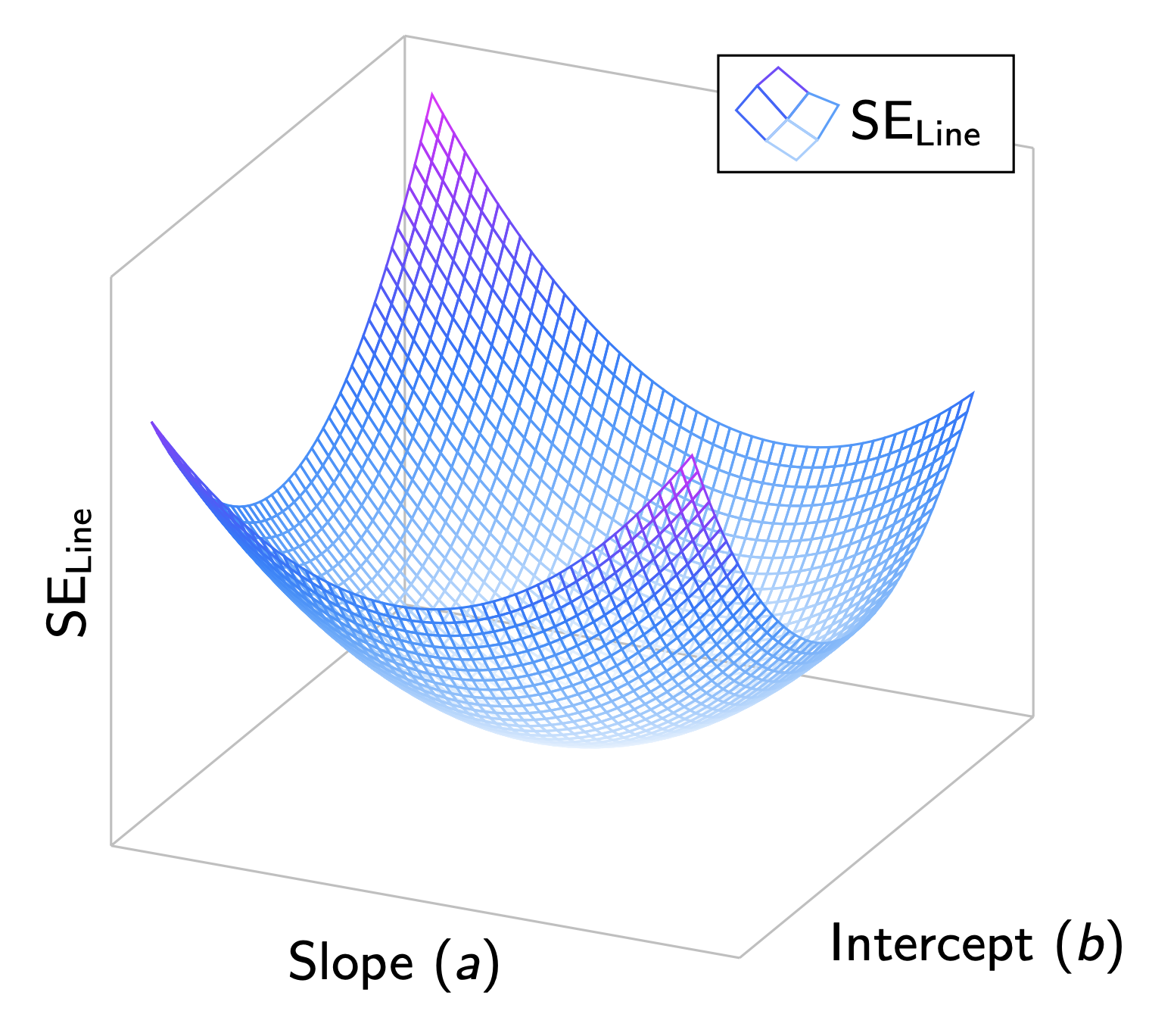
In the video, the residual sum of squares was shown as a heatmap and the arrows were used to represent the negative gradients. Here I just want to use a Z-axis to represent the residual sum of squares, such that I have:
- The X-axis: the slope
- The Y-axis: the intercept
- The Z-axis: the residual sum of squares
In addition, I have to use pgfplots to make the visualisation to have a consistent look with other content of the slides. What would the plot eventually look like? Let’s see.
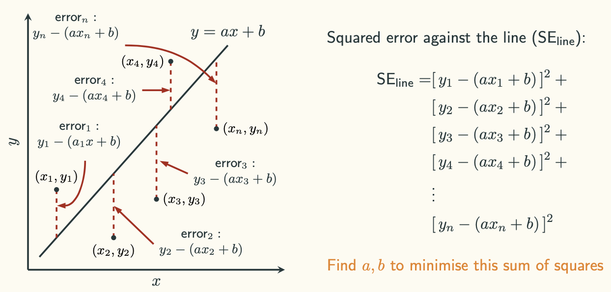
First, we need to clearly define what we actually want when we fit a straight line on a bunch of data points. In this case, we are doing a simple linear regression, and the method we are using is ordinary least square, or OLS. In OLS, it is the sum of the squared distance between the actual data point and the point on the line that we care about. Let’s denote this as $\text{SE}_{\text{line}}$, and

Basically, we are doing some computations in the following order:
- We generate some $(x_i,\ y_i)$ pairs with a linear relationship
- We represent a line in the form: $y=ax+b$
- We compute the $\text{SE}_{\text{line}}$:
$$ \text{SE}_\text{line} = \sum_{i=1}^n [y_i - (ax_i+b)]^2 $$
- We put the slope ($a$) as the X-axis, the intercept ($b$) as the Y-axis, and the $\text{SE}_{\text{line}}$ as the Z-axis. Plot their relationship. Note that $x_i$ and $y_i$ are the knowns, and $a$ and $b$ are the unknowns
We can further manipulate the expression of $\text{SE}_{\text{line}}$ to make it a bit clearer. Bear in mind that $a$ and $b$ are the unknowns:
$$ \begin{aligned} \text{SE}_\text{line} &= \sum_{i=1}^n [y_i - (ax_i+b)]^2\\[10pt] &= \sum_{i=1}^{n}[,y_i^2-2y_i(ax_i+b)+(ax_i+b)^2,] \\[10pt] &= \sum_{i=1}^{n}(y_i^2-2ax_iy_i-2by_i+a^2x_i^2+2abx_i+b^2) \\[10pt] &= \sum_{i=1}^{n}y_i^2-2a\sum_{i=1}^{n}x_iy_i-2b\sum_{i=1}^{n}y_i+a^2\sum_{i=1}^{n}x_i^2+2ab\sum_{i=1}^{n}x_i+nb^2\\[10pt] &= \sum_{i=1}^{n}y_i^2- \left(2\sum_{i=1}^{n}x_iy_i\right) \cdot a - \left(2\sum_{i=1}^{n}y_i\right) \cdot b + \left(\sum_{i=1}^{n}x_i^2\right) \cdot a^2 + \left(2\sum_{i=1}^{n}x_i\right) \cdot ab +nb^2 \end{aligned} $$
Now let’s get some data, say 25 data points. We do this in python:
import numpy as np

np.random.seed(42)
xs = np.random.normal(size=25)
ys = 2*xs + 1 + np.random.normal(size=25)
With xs and ys values, we can calculate the coefficients in the $\text{SE}_{\text{line}}$:
| Coefficient | Value |
|---|---|
| $\sum_{i=1}^{n}y_i^2$ | $135.95$ (sum(ys * ys)) |
| $2\sum_{i=1}^{n}x_iy_i$ | $96.60$ ( 2 * sum(xs * ys) ) |
| $2\sum_{i=1}^{n}y_i$ | $19.28$ ( 2 * ys.sum() ) |
| $\sum_{i=1}^{n}x_i^2$ | $22.63$ ( sum(xs * xs) ) |
| $2\sum_{i=1}^{n}x_i$ | $-8.18$ ( 2 * xs.sum() ) |
| $n$ | $25$ |
Now we have the function we want to plot:
$$ \text{SE}_\text{line} = 135.95 - 96.6a -19.28b + 22.63a^2 -8.18ab +25b^2 $$
In terms of the X-, Y- and Z-axes, we are plotting:
$$ z = 135.95 - 96.6x -19.28y + 22.63x^2 -8.18xy +25y^2 $$
Now we could plot the above function as a 3D mesh using \addplot3 from pgfplots. After playing around with the view{}{} option and setting appropriate domains of x and y, we can get a beautiful plot:

By looking at the this plot, it is clear to us that in OLS the $(a,b)$ we are looking for is the lowest point of the 3-dimensional parabola. The code used to generate the above plot is shown below:
\documentclass{beamer}

\usepackage{tikz}
\usepackage{pgfplots}

\begin{document}

\begin{frame}{OLS}
    \footnotesize
    \begin{tikzpicture}
        \begin{axis}[view = {25}{25},
                        xmin=-22.5, xmax=24, ymin=-23, ymax=22,
                        height=7cm, width=7cm,
                        axis line style={gray!50},
                        xtick=\empty, ytick=\empty, ztick=\empty,
                        xlabel={Slope ($a$)}, ylabel={Intercept ($b$)}, zlabel={$\text{SE}_{\text{Line}}$},
                        colormap/cool]
            \addplot3[mesh, samples=50, domain=-20:20, domain y=-22:21]
                        {135.95 - 96.6*x -19.28*y + 22.63*x^2 -8.18*x*y +25*y^2};
            \addlegendentry{$\text{SE}_{\text{Line}}$}
        \end{axis}
    \end{tikzpicture}
\end{frame}

\end{document}