ATAC-seq is THE simplest genomic protocol to profile open chromatin regions in the genome. The original publication (Nature Methods 10, 1213-1218) has been cited 441 times at this moment of writing (1,073 times at this moment of re-posting). It has become almost a routine for a lab that is interested in transcriptional regulation.
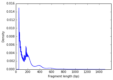
One common QC for the data is to plot the fragment size density of your libraries. The successful construction of a ATAC library requires a proper pair of Tn5 transposase cutting events at the ends of DNA. In the nucleosome-free open chromatin regions, many molecules of Tn5 can kick in and chop the DNA into small pieces; around nucleosome-occupied regions, Tn5 can only access the linker regions. Therefore, in a normal ATAC-seq library, you should expect to see a sharp peak at the <100 bp region (open chromatin), and a peak at ~200bp region (mono-nucleosome), and other larger peaks (multi-nucleosomes). Examples from one of my data:
Regular scale:
Log scale:
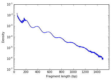
This clear nucleosome phasing pattern indicates a good quality of the experiment.
Different people probably have different ways of plotting this using different codes, but making this plot can be simply achieved by a combination of one line of unix commands and Excel. You don’t need some complicated scripts to do it at all.
The 9th column of sam/bam file contains the fragment length information of the paired reads. Therefore, you can count them by:
samtools view ATAC_f2q30_sorted.bam | awk '$9>0' | cut -f 9 | sort | uniq -c | sort -b -k2,2n | sed -e 's/^[ \t]*//' > fragment_length_count.txt
This is what it does:
samtools view ATAC_f2q30_sorted.bam | #stream reads

awk '$9>0' | #output reads with positive fragment length, i.e. left-most reads

cut -f 9 | #get the fragment length

sort | uniq -c | #count the occurrence of each fragment length

sort -b -k2,2n | #sort based on fragment length

sed -e 's/^[ \t]*//' #remove leading blank of the standard output
In the output, the 2nd column is the fragment length, and the 1st column is the counts. Open fragment_length_count.txt with Excel, and simply plot the 2nd column against the 1st column:
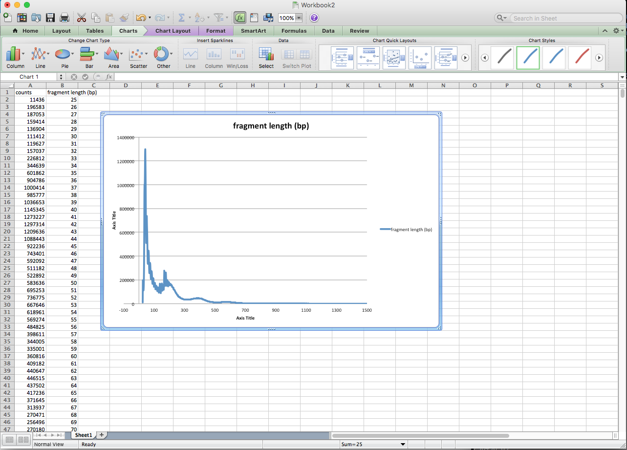
Okay, I guess this is not really about ATAC-seq, it is more about command line usage, and I admit, it is not as beautiful as the plot generated by matplotlib or R.
This is kind of like a histogram with 1-bp bin, which sometimes could be very spiky without smoothing.
In addition, many beginners don’t know what to expect from the library profiles (before sequencing) when running on a gel or Bioanalyzer/tapeStation etc. From our experience, we often see at least three peaks:
- The sharp peak around 200 bp, representing the open chromatin;
- The peak around 350 bp, representing mono-nucleosome;
- The peak around 550 bp, representing di-nucleosome;
Sometimes, we also see more peaks larger than 550 bp (not always). It could be a combination of large tagmented fragments and the artefacts of the Bioanalyzer (it is not a normal log scale like agarose gel). Click here to see a few examples of Bioanalyzer profiles from successful ATAC-seq experiments. Check the pdf files with names rep{1..10}_bioanlayzer.pdf. Note those are libraries where the Illumina Nextera adapters (136 bp) have been added.